Quantifying Meaning

Intro to Computational Semiotics: Part Three

Feb 2026

This is the third article in a 6-part series, where I break down "Intro to Computational Semiotics" lectures by Brandon Duderstadt (@calco_io on X).

In Part One, I broke down the first lecture, in which Brandon provided an overview of the history of philosophy relevant to the field of Computational Semiotics.

In Part Two, Brandon introduced foundational ML and linear algebra concepts through the lens of a linear autoencoder, building up to the tools that will be needed to understand the rest of the series: graphs, compression, loss functions, model space, and adjacency spectral embedding.

Part Two gave us the math, and in this third part we take a mechanistic look "under the hood." You can watch the lecture recording here.

For the non-technical reader: as with Part Two, the architectural details matter less for you than tracking the general trajectory of the series. The main idea I want to come through: these systems learn meaning from human language at scale, and "quantifying meaning" to make decisions about what counts as "equivalent meaning" is now an engineering choice with real consequences.

I. The Architecture of the Meaning-Making Machine

The system that most of us interact with daily when we use ChatGPT, Claude, or any other large language model is called a transformer. The transformer architecture was introduced in 2017 in a paper called "Attention Is All You Need."¹ It has remained the dominant language model architecture since.

Brandon relays an anecdote about the authors of the original paper. Aiden Gomez, one of the co-authors, is sitting on the couch with Ashish Vaswani after they've submitted the paper, and says something like, "We improved the benchmark score on this translation task by a couple points. Who's going to care?" Ashish responds: "Everyone will care, because this architecture is so simple. It's incredibly easy to scale it up."

As we saw with the model space discussion from Part Two, if you can take an architecture and scale it up to represent many functions with a ton of data, "suddenly you can win the prize."

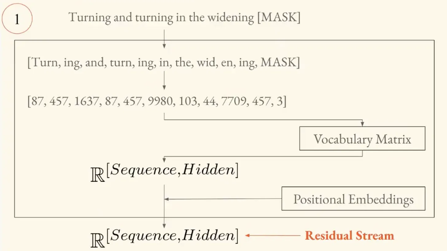
One distinction Brandon makes here is that the GPT paradigm (Generative Pre-trained Transformer) is separate from the transformer architecture. GPT refers to a specific way of training a transformer, where you take a corpus of text, mask the last token in a string, run the sequence through the model, and get a learning signal from how well the model predicts what that masked token is.

The Residual Stream

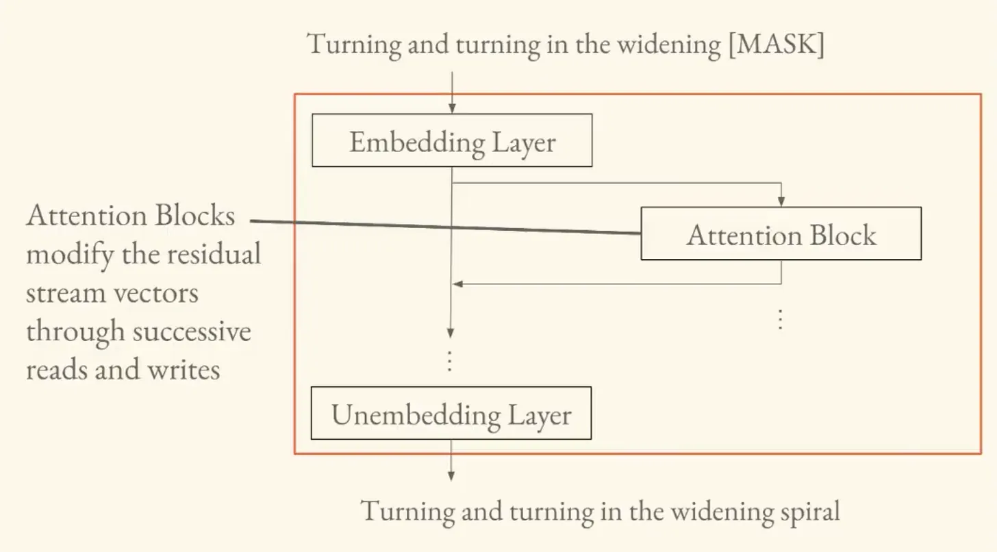
Brandon walks through the transformer by taking us into each of its layers, and teaching us about the transformations occurring at each one.

There are three:

1. The embedding layer
2. The attention blocks
3. The unembedding layer.

The embedding layer takes a sequence of text and converts it into vectors the model can operate on. This sequence of vectors is called the residual stream, which is at the center of the modern understanding of how transformers work.

As mechanistic interpretability research has progressed, researchers have realized that what's really going on inside the models is:

"You have attention heads that read from and write to these vector representations of your text in an iterative process."

The residual stream is like a central highway. Information enters as text, gets converted to vectors, and then attention blocks read from it, allow tokens to interact with each other, and write information back to it.

Attention as a Graph

Here we connect back to Part Two's discussion on graphs.

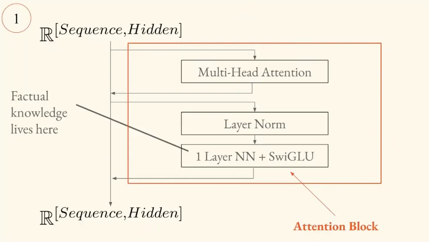
Inside each attention block, the sequence of token vectors gets projected through three linear layers called Q (query), K (key), and V (value). Q and K projections define a graph over your words. When the Q representation of one token is close to the K representation of another, those two tokens exchange information.

"This is in fact defining a graph on all of our tokens. The entry at every single position in that matrix tells you how much those two tokens are interacting. So every single layer in the transformer you have this directed graph that is defining how the information is going to mix."

The operation:

1. Build a graph that defines who each token is going to talk to.
2. Send specific information along the edges of that graph.

This fundamental operation occurs again and again to build up meaning within the models.

Every time you use a language model, a directed graph gets constructed over your words, deciding which tokens "talk" to each other.

The model also has multiple attention heads operating in parallel, each specializing in different operations. Some of these are copy heads (move tokens around), some are induction heads (make predictions), and some handle vocabulary or syntax. Others don't do much at all. An active area of research is to figure out what each head is responsible for and how that changes as you train models.

Where Does Fact Live?

After the attention block, there's a "feed-forward block," structurally similar to the autoencoder discussed in Part Two (but inverted). The autoencoder compresses information through a smaller hidden layer, while the feed-forward block expands it. The hidden layer has many more neurons than the output.

Brandon references a paper called "Locating and Editing Factual Associations in GPT"² (known as the "Rome paper"). The authors showed that you can identify exactly where factual knowledge is stored in the model by intervening in the weights of these feed-forward layers, and you can edit it this way.

"They're able to modify a transformer's understanding of factual knowledge... they're able to identify exactly where that factual knowledge is stored in the model and edit it so that the model returns Rome when asked [about the capital of France]."

The attention blocks look at the context of your language and update their understanding of what words mean based on that context. The feed-forward layers then retrieve factual knowledge obtained over the course of training to enrich the model's understanding of the meaning of that language.

The Objective

The transformer is trained to predict the next word. Its loss function, softmax cross-entropy, can be summarized as "maximize the probability of the correct next token."

Brandon invokes a quote from Ilya Sutskever, a former chief scientist at OpenAI who now runs his own lab:

"Predicting the next token well enough means that you understand the underlying reality that led to the creation of that token."

Ilya's argument is that as you get better at predicting what comes next in language, you're forced to build up internal models of increasingly sophisticated phenomena. Early training needs grammar. Then you need to model the rough subject of a text. Then you hit stories, and suddenly you need to understand narrative. You hit math textbooks, and suddenly you need mathematics.

A philosophical question arises: how does prediction relate to "understanding?"

II. Measuring Meaning at Scale

From transformers, Brandon moves to the embedding models. Transformers create one vector per token (to predict the next word). Embedding models create one vector per document. If two documents have similar meanings, their vectors should be close together.

Embedding models are the main tool we have for manipulating unstructured data computationally, whether that's text, images, video, or audio. For Computational Semiotics, they're the instruments that let us actually measure semantic similarity at scale. If you want to track how meaning shifts across a social network over time, you embed the documents and watch the vectors move.

Early vs. Late Interaction

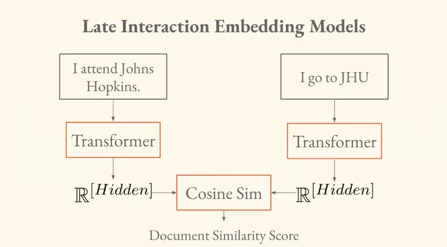
Brandon introduces two paradigms for comparing documents.

1. Early interaction. You pass both documents into the same model together, and the model outputs a similarity score. This works, but it requires passing every pair of documents through the model. If you have a massive dataset, that's n-squared model invocations. Not feasible.
2. Late interaction. You run each document through the model once, independently, and get a vector for each. Then you compute similarity between vectors after the fact. This only requires a linear number of passes.

III. Decisions On Meaning

Embedding models learn through contrastive training, where you take pairs of documents you consider "semantically equivalent," embed them, and try to make their vectors close together while pushing apart vectors for unrelated documents.

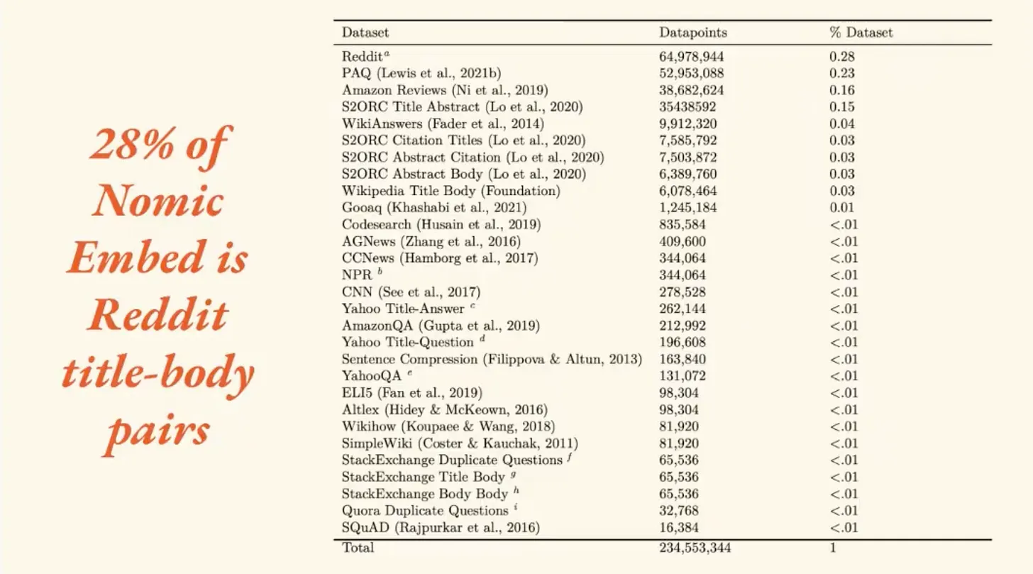
Brandon uses Nomic Embed, which at the time was the most performant embedding model in the world, as a case study.³ The training data breakdown was:

• 28% Reddit title-body pairs
• 23% Q&A pairs (from a dataset called PAQ)
• Remainder scraped from across the internet

Real data from the training set included a Reddit post titled: "The one feature that iPad is really missing." The body is a "tirade" about things the user doesn't like. Brandon says:

"It's super unclear to me that these are semantically equivalent. Like this one is kind of a clickbait title. And this is a tirade about various aspects of the Apple ecosystem."

Regarding the Q&A pairs: if you have a question and its answer, are those two things expressing the same reference with different senses? Or is the situation closer to two similar questions being closer to each other, with the answer as their shared reference?

Frege's Sense and Reference problem from Part One is now an engineering decision with semiotic consequences. The definition of "equivalence" you choose shapes what the model learns about meaning itself.

More on Language Games

Brandon identifies that the model is being asked to play different language games. There's the similarity game (how close are these two questions?) and the question-answering game (can you find the answer to this question?). These are fundamentally different tasks to disambiguate.

This framing is Wittgensteinian, connecting back to the language games discussion from Part One. The solution in Nomic Embed was: for every sequence in the training data, they tell the model which "game" it's playing.

Four Innovations

Brandon details four innovations in how Nomic Embed was built:

1. Data curation: Train a rough "poor model" on all the data, use it to score pairs, and throw away the ones it flags as dissimilar.
2. Task disambiguation: Tell the model explicitly whether it's playing the similarity game or the question-answering game.
3. Efficient sampling (GradCache): Find ways to compare against more negative samples at training time without running out of memory.
4. Hard negative mining: Not all negative examples are equally useful. "I go to school in Baltimore" is a much harder negative for "I go to Johns Hopkins" than "I like coffee" is. You want hard negatives, but you also have to be careful not to accidentally mine false negatives (things that actually are semantically equivalent but aren't labeled as such in your data).

IV. Imperfect Instruments

The loss function for Nomic Embed is called "InfoNCE." In a standard transformer, cross-entropy loss compares the model's prediction against every possible token in the vocabulary. InfoNCE takes an economical approach in comparing against a sample of negatives.

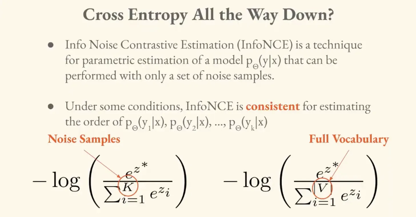
If you're trying to pick the most probable next token, you don't need to model the full probability distribution perfectly.

"It doesn't matter if we say the probability of 1997 here is 0.8 or 0.82 or whatever, as long as it's higher than everything else."

Technically you'd need infinitely many samples for convergence, which isn't achievable. However, getting as many as possible as efficiently as possible gets you "close enough."

This is a principle for the field of Computational Semiotics broadly. The instruments for semiotic measurement are inherently imperfect. They only need to be good enough to meaningfully track the changes we care about.

The innovations in how we build them reveal something about the nature of the problem, which is that meaning is context-dependent and contested. The engineering decisions we make about what counts as "the same meaning" are themselves semiotic acts.

Brandon ended the lecture by previewing lecture four on "Information Cartography" and dimensionality reduction. How do we take these high-dimensional meaning spaces and make them visible?

In Part Four, we'll look at how you map the terrain.

So Long,

Marianne

¹

Ashish Vaswani et al., "Attention Is All You Need," arXiv:1706.03762 (2017), https://arxiv.org/abs/1706.03762

²

Kevin Meng et al., "Locating and Editing Factual Associations in GPT," arXiv:2202.05262 (2022), https://arxiv.org/abs/2202.05262

³

Zach Nussbaum et al., "Nomic Embed: Training a Reproducible Long Context Text Embedder," arXiv:2402.01613 (2024), https://arxiv.org/abs/2402.01613