Intro to Computational Semiotics: Part Two

Jan 2026

This is the second article in a 6-part series, where I break down “Intro to Computational Semiotics” lectures by Brandon Duderstadt (@calco_io on X).

In Part One, I broke down the introductory lecture in which Brandon provided an overview of the history of philosophy relevant to the field of Computational Semiotics.

I introduced an argument that I want to highlight again as a framing device:

In the age of generative AI, our language may be subject to mass modification — whether via deliberate engineering or emergent shifts from widespread usage. Either way, how we make meaning is shifting at scale. Language is becoming something actively shaped by the tools we use to produce it.

Instruments for Measurement

It’s important for us to track and measure these changes computationally, because they are happening at a speed and scale beyond human observation. The changes are also computational in origin, resulting from the AI systems adopted into our daily knowledge work. This is the case for the importance of Computational Semiotics.

In this second lecture, Brandon introduces some foundational ML/linear algebra concepts necessary for the tools of the trade, or the instruments we actually use to measure language for this purpose.

For the non-technical reader: you don’t need to worry about tracking every detail here, just the shape of the argument.

The lecture doesn’t get into the direct methodologies for Computational Semiotics — the goal is to give a brief overview of the advanced concepts and vocabulary to draw upon later in the class.

Brandon builds up the fundamentals through the lens of training a neural network called a linear autoencoder. Autoencoders are:

a special type of neural network that learn to compress data into a compact form and then reconstruct it to closely match the original input. They consist of an:

Encoder that captures important features by reducing dimensionality.

Decoder that rebuilds the data from this compressed representation.¹

I’ll run through each of the concepts he introduces through this worked example.

I. Setup: Graphs & Forward Propagation

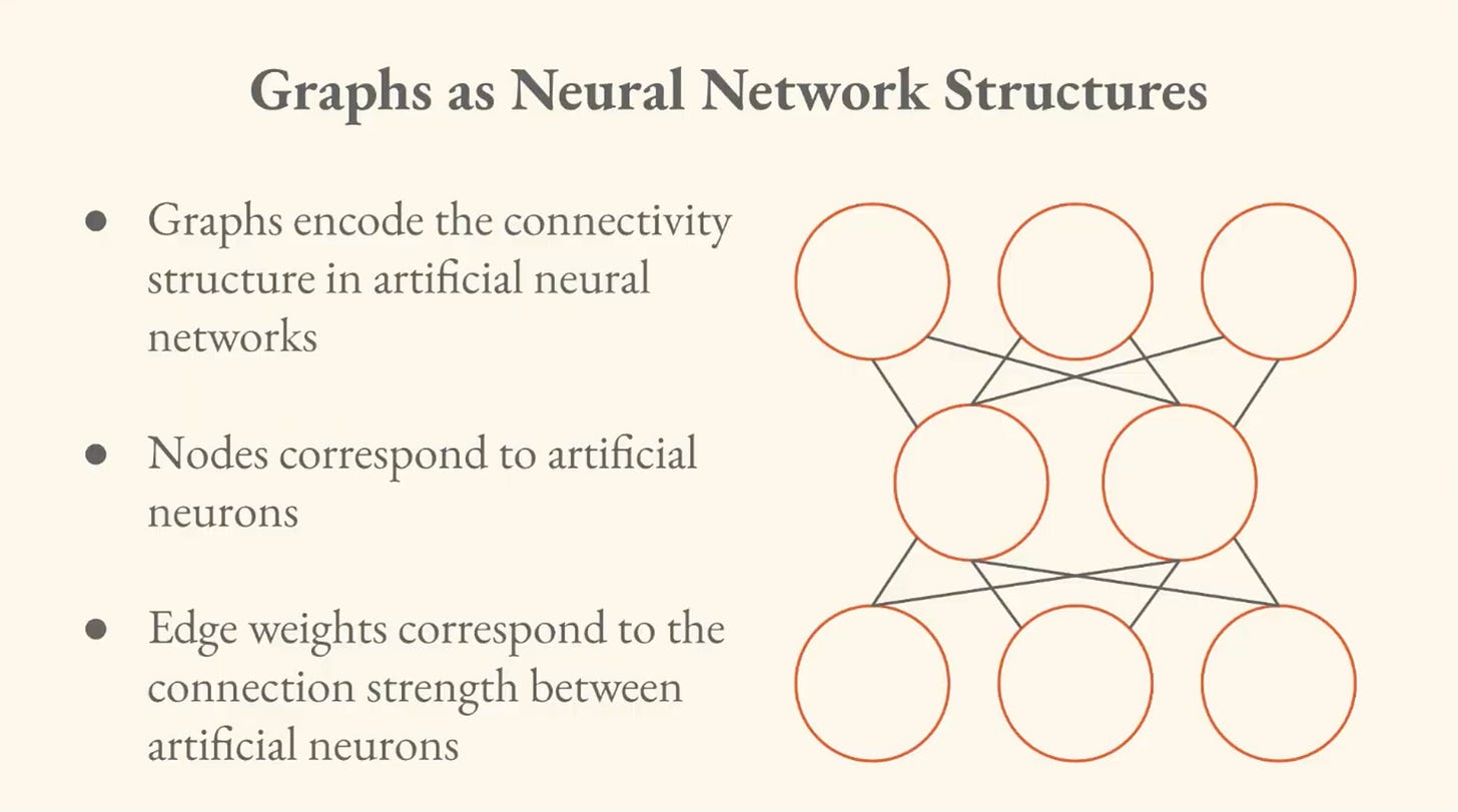
The most fundamental abstraction is a Graph, defined as a set of vertices and a set of edges. There are nodes which represent some entity we are trying to model, and edges that connect those nodes.

The Graph was initially developed to try to understand, for a variety of land masses and peninsulas and bridges, whether all the bridges could be crossed exactly once without retracing any steps.

Now we use them for myriad contexts, from social network graphs to transit graphs to brain graphs.

In a social graph, like a graph of relationships on X, the nodes may represent users and the edges are the connections between them (like followed/following).

Graph Matrix Correspondence

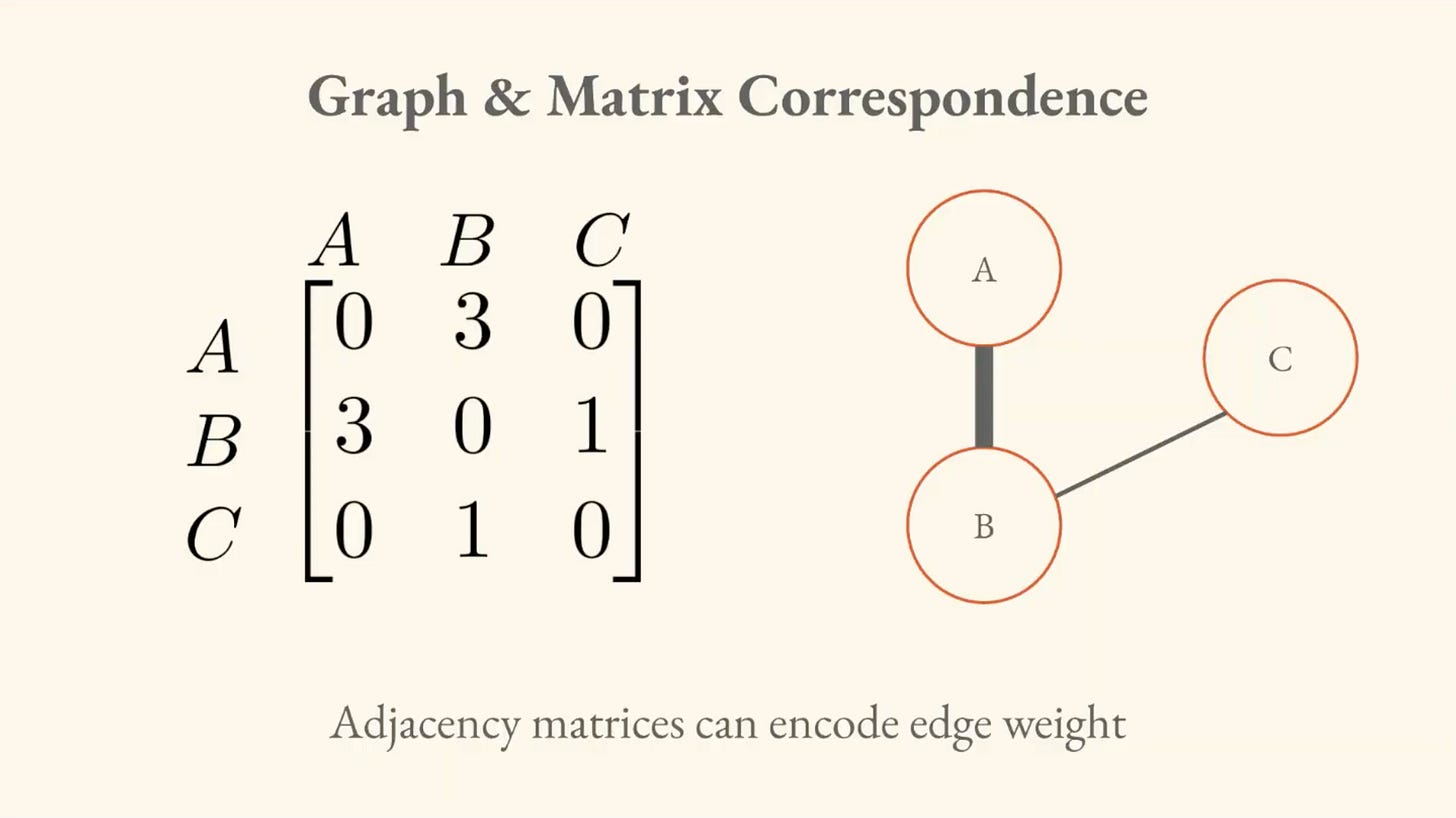
You can take the information in any graph and summarize it in an adjacency matrix. This allows us to operate on graphs computationally. We can transform questions about the graph into questions about the properties of the adjacency matrix. We operate on these objects with linear algebra.

We can encode things like the direction of the relationship, as well as the strength of the connection (edges have “weights”).

In the example of the linear autoencoder, this model represents artificial neurons (the nodes) and the strengths between them (the edges).

All of this information can, again, be wrapped up into a matrix.

Each number corresponds to a strength of connection between the artificial neurons.

Forward Propagation

In forward propagation through a neural network, you have an input signal (often represented as a vector, a sequence of numbers) and we can look at how the signal is going to move through the structure computationally.

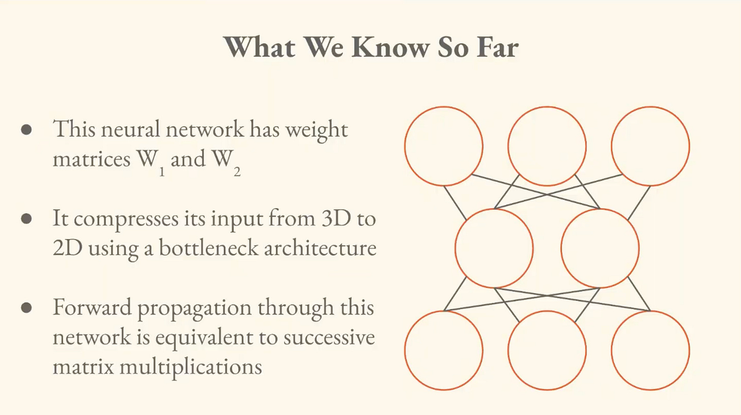
So we have the input layer of neurons, a hidden layer in the middle, and an output layer. Through successive matrix multiplication, we can model moving the signal through the graph.

We may also want to look at other correspondences between these neurons.

Column Space & Rank

In our neural network interpretation, we’ll define the column space as the set of all possible outputs that could be generated by forward propagating through it. Rank is the dimension of the column space.

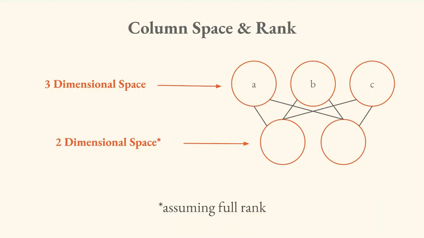
The column space tells you what outputs are possible given the network’s structure. The rank tells you the dimensions of those outputs. If you push 3D data through a 2D bottleneck, the rank is at most 2, because information gets compressed.

I don’t want to get too into the weeds here, but the main thing to understand is these three layers:

Input Layer: This is where the original data enters the network. It can be images, text features or any other structured data.

Hidden Layers: These layers perform a series of transformations on the input data. Each hidden layer applies weights and activation functions to capture important patterns, progressively reducing the data’s size and complexity.

Output (Latent Space): The encoder outputs a compressed vector known as the latent representation or encoding. This vector captures the important features of the input data in a condensed form [and] helps in filtering out noise and redundancies.²

Remember the connection between Plato’s Cave and projection in linear algebra from the first lecture? The “hidden layer” in the neural network is like the cave wall. The network can only express a flat (2D) shadow of the original, higher-dimensional input.

II. How the Network Learns

This is the most detailed section, and I’ll introduce some of the concepts from it briefly.

Brandon says that it’s a bit useless to have a model of a neural network if you can’t get it to do anything, so he walks us through “the ingredients” for how the network learns.

The Foundational Concepts

Training Dataset

Usually represented as another matrix. Because the input dimensionality of the neural network we’re looking at is three, there are three features in the training dataset:

X ∈ ℝ^[N,3]

N denotes the number of samples.

Loss Function

This defines the behavior of the network, during training and in terms of what you’re trying to get it to do after training. The loss function takes the output of the network and attempts to compress it down to a single number — a scalar — and this number is high when your network is doing a bad job at what you want it to do, and low when it is doing a good job.

Relevant aside — Brandon gives an anecdote of running into Oriol Vinyals at a conference and receiving this advice, which seems worth repeating:

“The most important thing you can possibly do, in all endeavors, is understand your objective function . . . because everything else flows down from that.”

We can understand how good or bad of a job the network is doing, but how do we actually change it to do better at the task we’ve specified? That is where an optimizer comes in.

Optimizer

Put simply, the optimizer is the rule for reducing loss. It’s how the network learns from its mistakes. You take the loss of the current output and figure out how much, and in which direction, to adjust the weights to improve the performance of the network with respect to the specified task.

“It uses your data to traverse model space to find better and better models.”

What is model space, then?

Model Space

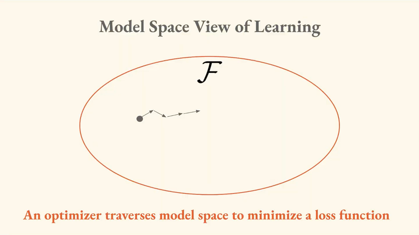
The model space is the set of all possible models that can be expressed by a given architecture and parameterization. For our neural network, this is the set of all possible functions that it can compute. The model space is formed by all possible configurations of parameters that can be put into the network.

A model space, loss function, and optimizer produce an estimation procedure.

Common Problems with Model Space

Misspecification: The correct model is not in your model space. In this case, our model is “misspecified.”

Procedure bias: Your estimation procedure may converge to a systematically incorrect model. This can come from the optimizer itself, which might steer learning toward certain regions of model space even when there are better solutions.

Sample insufficiency: The correct model is in your model space, but it’s too far away for you to reach with your finite dataset.

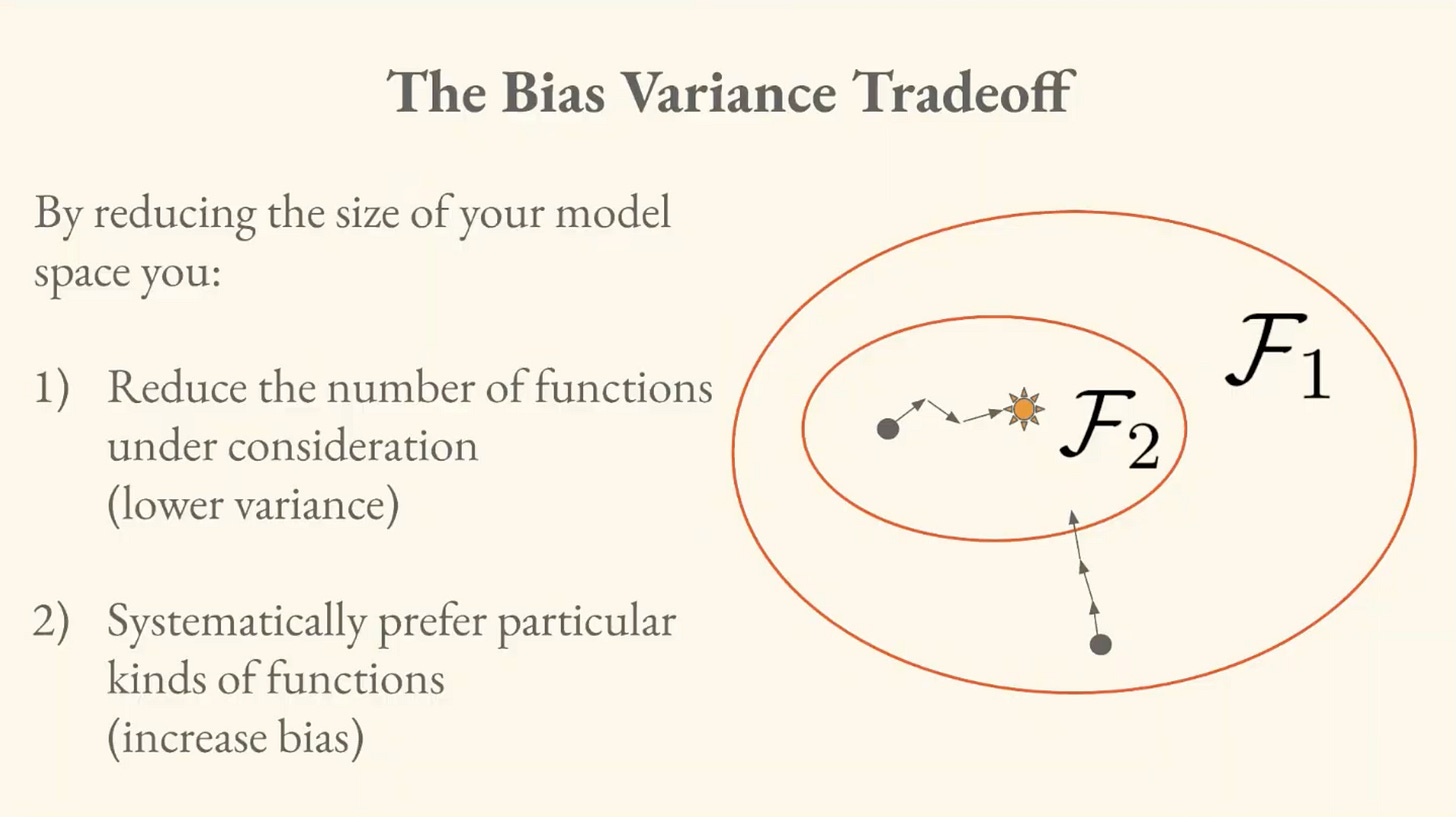
A smaller model space gives you more stability, but it might be systematically wrong (bias). A larger model space gives you more expression but it’s sensitive to noise in your dataset (variance).

A Model Space View of Modern AI

“Let’s use as much data as possible and consider as many functions as possible.”

By increasing the amount of data and the size of their models, Kaplan et al. found that the error kept going down in a predictable way. From this we got the “scaling era” which has been the state of AI for the past several years.

Brandon brings up a paper called “The Platonic Representation Hypothesis”³ which was based on the fact that neural networks trained on different datasets with different objectives converged on a shared statistical model of reality.

He argues, however, that training models on basically identical data (the entire internet) != making a statement about the Platonic world of forms.

III. Payoff: Solving the Autoencoder

As a reminder, the neural network we’ve been looking at throughout this lecture is a linear autoencoder.

The problem to solve with the autoencoder is:

Given three-dimensional dataset X, what are the optimal weights that minimize the reconstruction error when it passes through the two-dimensional bottleneck of the hidden layer?

The optimal weights are given by the Singular Value Decomposition (SVD) of the data matrix. The math and technical aspects are probably beyond the scope of this article, but you can just remember that SVD finds the directions in your data with the most variance, so you can throw away the rest and keep what matters.

“What else can we hit with the SVD hammer?”

The autoencoder was just a lens through which we could look at these foundational concepts. Where else does optimal compression matter, especially as it relates to Computational Semiotics?

This is where Brandon brings us back to Graphs, which is how he opened the lecture. SVD is optimal linear compression. Where else can we apply this? Graphs.

We gave the example of the social network as a possible model that can be represented by a graph. You can represent a social network as an adjacency matrix. From there, Adjacency Spectral Embedding (ASE) uses SVD to assign each node a vector that captures its position in the network structure.

The Computational Semiotics Connection

We’ll be looking at how language flows through social networks. In memetics, we look at how memes propagate through networks. We learned in lecture one that we care about how meaning shifts and changes as it passes from node to node. ASE lets us turn the network structure into something we can study computationally.

This means we have tools to track how meaning travels over time. You can embed a social network, look at clusters of relationships and meaning formation, and watch the network as it evolves, to answer Computational Semiotics questions.

In Part Three, we’ll begin to look at ways to quantify meaning, using these tools and concepts as foundations for this work.

Until then, if you’d like to preview Brandon’s third lecture and learn along with me, you can watch it here.

So Long,

Marianne

“Auto-Encoders,” GeeksforGeeks, https://www.geeksforgeeks.org/machine-learning/auto-encoders

Ibid.

Minyoung Huh, Brian Cheung, Tongzhou Wang, and Phillip Isola, "The Platonic Representation Hypothesis," arXiv:2405.07987 (2024), https://arxiv.org/abs/2405.07987